===============================================
Introduction
In traditional finance, Jensen’s alpha is a widely recognized measure of risk-adjusted performance, used to evaluate whether a portfolio generates excess returns relative to its expected performance based on the Capital Asset Pricing Model (CAPM). However, in the rapidly growing world of cryptocurrency derivatives, particularly perpetual futures, the calculation and interpretation of Jensen’s alpha differ significantly from its classical application in equities and bonds.
Perpetual futures introduce unique features—such as funding rates, 24⁄7 trading, and crypto-specific volatility—that challenge traditional assumptions about market returns and risk-free rates. This makes it essential for investors, traders, and quantitative analysts to understand how Jensen’s alpha differs in perpetual futures and how it can still serve as a valuable performance evaluation tool.
This article provides a comprehensive exploration of the concept, compares methodologies, highlights advantages and limitations, and shares practical insights into applying Jensen’s alpha in perpetual futures strategies.
What Is Jensen’s Alpha?
Traditional Definition
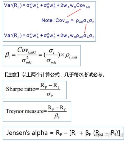
Jensen’s alpha measures the excess return a portfolio generates beyond what CAPM predicts. The standard formula is:
α=Rp−[Rf+β(Rm−Rf)]\alpha = R_p - [R_f + \beta (R_m - R_f)]α=Rp−[Rf+β(Rm−Rf)]
Where:
- RpR_pRp = portfolio return
- RfR_fRf = risk-free rate
- β\betaβ = sensitivity to the market portfolio
- RmR_mRm = market return
If alpha is positive, it suggests the manager or strategy generated returns beyond what was expected given its exposure to systematic risk.
Application in Equities and Bonds
In traditional markets, Jensen’s alpha is calculated against benchmarks like the S&P 500 or government bond indices, with stable risk-free rates such as U.S. Treasury yields.
How Jensen’s Alpha Differs in Perpetual Futures
1. Market Benchmarks
Unlike equities, perpetual futures lack a universal benchmark. Traders often use Bitcoin or Ethereum spot indices, crypto market-cap weighted indices, or synthetic indices built from major exchanges. This introduces benchmark risk, since the chosen market return may not reflect broader crypto conditions.
2. Risk-Free Rate Challenges
In perpetual futures, defining RfR_fRf is complex. Options include:
- U.S. Treasury yields (traditional proxy).
- Stablecoin yields on DeFi lending protocols.
- Exchange-provided funding rates, which act as implicit “carry costs.”
Each choice significantly affects the calculated alpha.
3. Funding Rates and Continuous Trading
Perpetual contracts charge or pay funding rates to keep futures prices aligned with spot. This creates a structural drag or boost to returns not present in traditional securities, altering the meaning of alpha.
4. Volatility Regimes
Crypto markets exhibit extreme volatility compared to equities. Standard beta calculations often underestimate tail risk. Consequently, Jensen’s alpha in perpetual futures needs volatility-adjusted benchmarks to avoid misinterpretation.
Traditional vs. perpetual futures alpha calculation differences.
Two Approaches to Calculating Jensen’s Alpha in Perpetual Futures
Method 1: CAPM Extension with Funding Rate Adjustment
This method adapts CAPM by including funding payments as part of the risk-free adjustment.
Formula adaptation:
α=Rp−[(Rf+F)+β(Rm−(Rf+F))]\alpha = R_p - [(R_f + F) + \beta (R_m - (R_f + F))]α=Rp−[(Rf+F)+β(Rm−(Rf+F))]
Where FFF represents the average funding cost (positive or negative).
Pros:
- More accurate in reflecting actual net returns.
- Widely applicable across major exchanges.
Cons:
- Sensitive to rapid funding rate fluctuations.
- Requires consistent funding data across venues.
Method 2: Factor-Based Model Approach
Instead of CAPM, traders use multi-factor models that include volatility indices (VIX-like measures), liquidity factors, and crypto-specific momentum factors. Jensen’s alpha becomes the residual return after accounting for these variables.
Pros:
- Captures crypto-specific risk drivers.
- More robust during market turbulence.
Cons:
- Requires complex data sets and statistical expertise.
- Less intuitive compared to CAPM-style alpha.
Recommendation: For retail traders and smaller funds, CAPM with funding adjustment is practical. For institutional investors, factor-based models provide superior accuracy in interpreting alpha.
Practical Applications of Jensen’s Alpha in Perpetual Futures
Portfolio Performance Evaluation
By calculating alpha, managers assess whether their trading strategy genuinely outperforms market expectations or merely tracks crypto beta.
Risk Management
For quantitative analysts and risk managers, Jensen’s alpha helps identify hidden risks not explained by market movements.
Strategy Optimization
Alpha can highlight whether systematic leverage, arbitrage strategies, or funding rate plays are driving performance.
This ties directly into how to calculate Jensen’s alpha in perpetual futures for advanced portfolio analysis.
Case Example: Jensen’s Alpha for a Bitcoin Perpetual Futures Trader
- A trader achieves 20% annualized returns trading BTC perpetual futures.
- Benchmark BTC spot index: 15%.
- Risk-free rate (U.S. Treasuries): 3%.
- Beta: 1.2.
- Average funding rate: -2% (cost).
α=20−[(3−2)+1.2×(15−(3−2))]=20−[1+1.2×14]=20−17.8=2.2\alpha = 20 - [(3 - 2) + 1.2 \times (15 - (3 - 2))] = 20 - [1 + 1.2 \times 14] = 20 - 17.8 = 2.2α=20−[(3−2)+1.2×(15−(3−2))]=20−[1+1.2×14]=20−17.8=2.2
This positive 2.2% alpha suggests the trader’s strategy outperformed market expectations even after funding costs.
Sample Jensen’s alpha calculation in perpetual futures.
Key Advantages and Limitations
Advantages
- Provides objective measure of outperformance.
- Can adjust for funding costs unique to perpetual futures.
- Useful for comparing strategies across markets.
Limitations
- Benchmark selection heavily influences results.
- Risk-free rate definitions in crypto remain unstable.
- Volatility distortions can mislead if not adjusted properly.
FAQ: Jensen’s Alpha in Perpetual Futures
1. Why is Jensen’s alpha significant in perpetual futures?
It allows traders and investors to distinguish between skill-driven returns and those explained by market exposure or leverage. This is crucial in crypto, where volatility can mask whether strategies truly add value.
2. How do funding rates impact Jensen’s alpha?
Funding rates act as implicit financing costs. A trader paying high funding may see alpha reduced even if raw returns are strong, while receiving funding can artificially boost alpha. Adjusting for this is essential.
3. Can Jensen’s alpha be used by retail traders?
Yes, but with caution. Retail traders can apply simplified CAPM-style alpha calculations using spot indices as benchmarks. However, for deeper insights, professional tools and factor-based models are recommended.
Conclusion
Understanding how Jensen’s alpha differs in perpetual futures is vital for both institutional and retail market participants. While the classical definition works in equities, perpetual futures require adjustments for benchmarks, funding rates, and volatility regimes.
By applying adapted CAPM models or advanced factor-based methods, traders can unlock a more accurate view of their strategies’ true performance. In the evolving crypto derivatives landscape, Jensen’s alpha remains an indispensable tool for measuring skill, risk-adjusted returns, and long-term sustainability.
Was this article useful in clarifying Jensen’s alpha in perpetual futures?
Leave a comment, share with your network, and join the conversation on advanced crypto performance metrics.
Would you like me to also prepare a step-by-step tutorial on Jensen’s alpha for perpetual futures so readers can calculate it with real market data?